NEM – Wind Generation Dashboard

Introduction & Context

The National Electricity Market (NEM) is increasingly shaped by the contribution of wind generation, particularly in Victoria. This dashboard provides a clear, near real‑time view of how the state’s registered wind farm fleet is performing, in both aggregate and individual sites.

At its core, the dashboard tracks four key dimensions of fleet activity:

• Registered sites – the total number of wind farms formally registered with AEMO.
• Reporting sites – those currently online and sending SCADA telemetry.
• Generating sites – farms actively producing electricity at the moment.
• Non‑generating sites – farms online but not dispatching power.

To capture both short‑term volatility and longer‑term patterns, the dashboard presents 24‑hour, 7‑day, and 30‑day views of wind output. These rolling windows highlight daily variability, weekly weather cycles, and monthly fleet utilisation trends.

For the latest snapshot, gauges provide an instant picture of each farm’s output relative to its registered capacity. Colour coding makes it easy to see which sites are performing strongly, which are idling, and which are curtailed. This design choice ensures that the story is not just about raw megawatts, but about capacity utilisation — how effectively the fleet is being used at any given time.

The aim is to move beyond abstract generation figures and tell a more narratable story: Is Victoria’s wind fleet being fully leveraged? Which farms are consistently contributing, and which are falling short? How does the fleet’s behaviour change across different time horizons? By combining gauges, colour codes, and time‑series views, the dashboard makes these questions visible and answerable at a glance.

Problem / Observation Goal

Wind generation has become a central contributor to Victoria’s renewable mix, but its dispatch profile is inherently variable — shaped by weather systems, turbine availability, and market signals. This dashboard filters SCADA data by fuel_primary = 'Wind' and region = 'VIC1', presenting both fleet‑level output and per‑unit traces.

The observation goal is twofold:

• Track the number of registered wind farms, the subset actively reporting telemetry, and those actually generating power versus idling.
• Compare behaviour across 24‑hour, 7‑day, and 30‑day windows, highlighting short‑term volatility and longer‑term utilisation trends.

A clear pattern emerges: wind output rises and falls with weather fronts, often peaking overnight or during storm events, then tapering in calmer conditions. Gauges and colour‑coded capacity percentages make this variability visible at a glance — showing which farms are consistently contributing and which are frequently offline.

The goal is not just to measure megawatts, but to narrate fleet utilisation: how often Victoria’s wind assets are engaged, how evenly they contribute, and how their collective behaviour supports or challenges grid stability. This diagnostic view complements the broader story of renewable integration, revealing both strengths and gaps in the state’s wind fleet

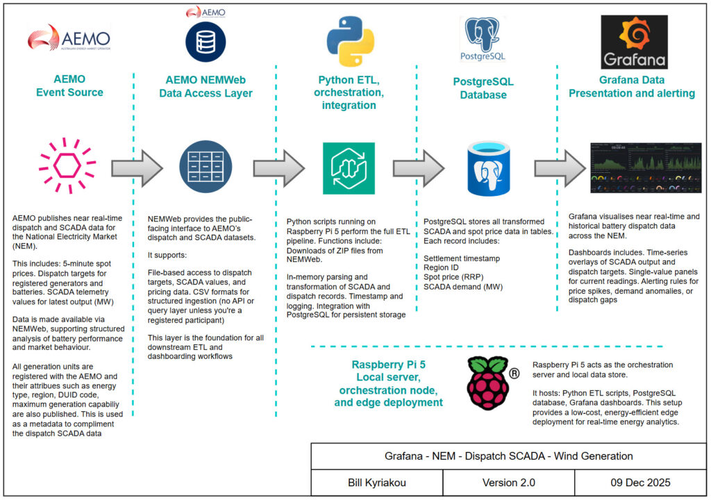
Data Sources & Collection

• Generation Source: Wind generation site accros the Victoria (VIC1) region.
• Data Source: AEMO Dispatch_SCADA dataset via NEMWeb
• ETL: Python script (GetStore_Dispatch_SCADA.py) running on Raspberry Pi 5
• Database: PostgreSQL storing timestamped SCADA records with DUID mapping
• Visualisation: Grafana dashboards with per‑unit gauges and stacked output traces
• Hardware: Raspberry Pi 5 acting as orchestration node and edge server

Design Philosophy & Dashboard Approach

The dashboard is designed to make wind’s variability narratable rather than overwhelming. Headline counts show how many farms are registered, reporting, generating, or idle, while time‑series views across 24‑hour, 7‑day, and 30‑day windows reveal both short‑term volatility and longer weather‑driven cycles.
Snapshot gauges and colour‑coded percentages of registered capacity provide instant recognition of which farms are contributing strongly and which are currently under‑utilised. Each panel serves a distinct role, counting for readiness, traces for variability, gauges for farm utilisation performance.

System Architecture

Data flow: NEMWeb → Python ETL → PostgreSQL → Grafana

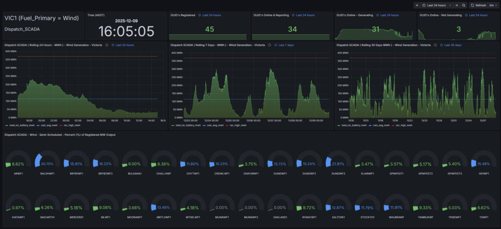
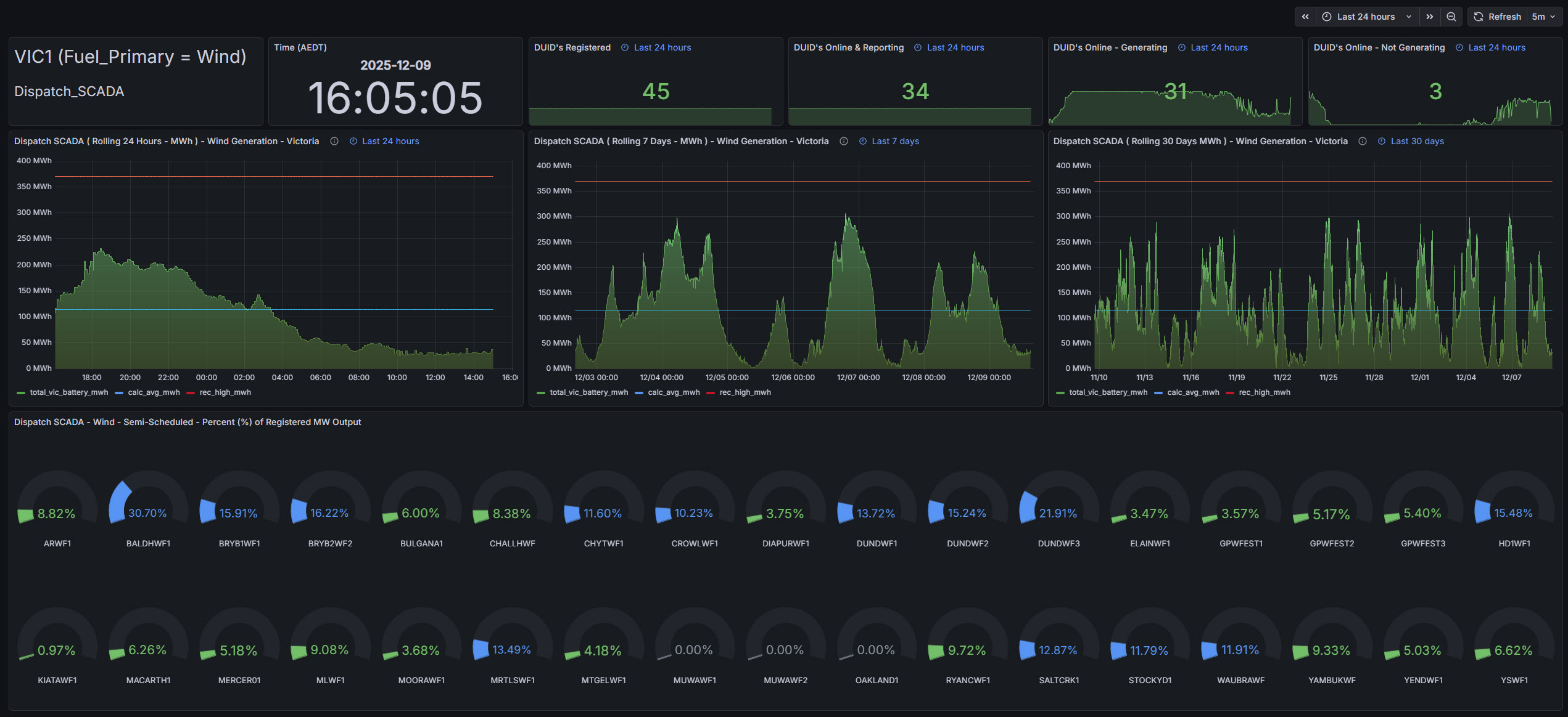
Dashboard Showcase

• Top panel: Circular gauges showing real‑time MW output and % capacity for each wind farm
• Bottom panel: Stacked area chart showing total wind output over time, segmented by farm
• Legend: Each farm trace colour‑coded for clarity and comparison
• SQL filters: Region = ‘VIC1’, Fuel Descriptor = ‘Wind’

Outcomes & Insights

• Dispatch visibility: Real‑time and historical wind output trackable per farm
• Fleet comparison: Gauges highlight which farms are active, idle, or curtailed
• Operational reliability: Raspberry Pi 5 and PostgreSQL ingest and serve data continuously
• SCADA transformation: Instantaneous MW values visualised directly and grouped by farm

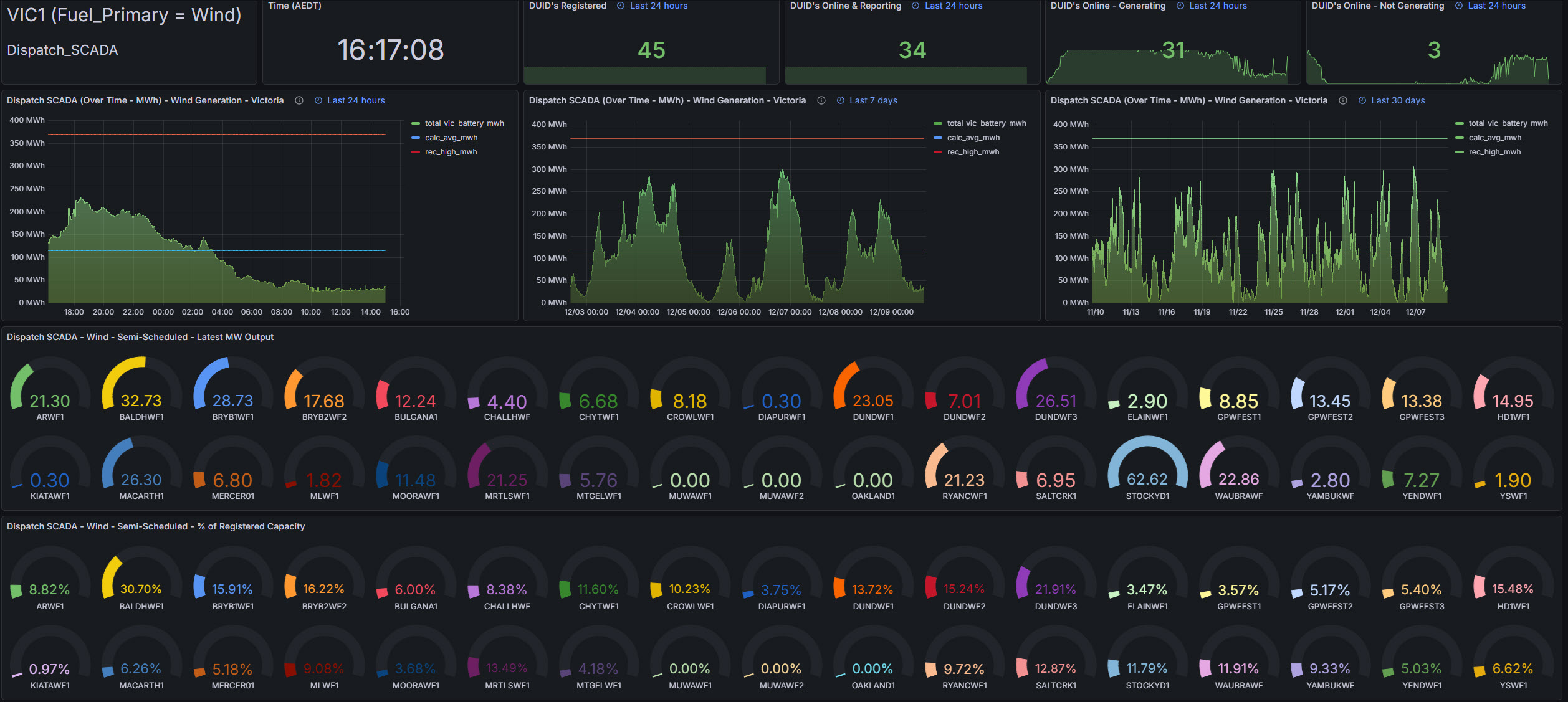
Lessons Learned

• Clarity beats complexity – Early versions of the dashboard tried to show everything at once — gauges, time series, counts, maps — but lacked a clear visual hierarchy. Viewers didn’t know where to look first. The fix was to anchor the layout around a single headline metric (Fleet Utilisation) and build supporting panels around it.
• Distraction kills momentum – Development was often interrupted by plugin errors, Grafana quirks, or chasing edge cases in SCADA data. Each detour delayed the core goal: narrating wind dispatch clearly. Lesson: isolate debugging from storytelling — fix the plumbing first, then build the narrative.
• Bad design hides good data – Circular gauges looked slick but didn’t scale. With 30+ wind farms, they became noisy and hard to compare. Replacing them with ranked bar charts made underperformers immediately visible. Lesson: choose visuals that serve the story, not the aesthetic.
• Not all data adds value – Including every DUID, every timestamp, and every metric created clutter. Some panels were technically correct but narratively useless. Lesson: if a panel doesn’t help explain dispatch behaviour or fleet performance, it’s out.
• The story matters more than the tech – The real goal isn’t showing MW values — it’s answering: Is Victoria’s wind fleet being used effectively? Are some farms consistently underperforming? Is dispatch behaviour predictable? Lesson: every panel should help answer those questions.
• Modularity enables reuse – By parameterising the dashboard for region and fuel type, the same layout now works for coal, wind, solar, batteries or any other registered generation technology. Lesson: build once, reuse everywhere.
• Narratability is a design constraint – Clients or stakeholders won’t read SQL or decode Grafana quirks. The dashboard must explain itself. Adding definitions, legends, and consistent labels turned a technical tool into a narratable product.
• Example of my old dashboard design that was revised to the dashboard above.

Future Development & Fixes

• Add nominal capacity metadata to enable dynamic % calculations based on either registered capacity or maximum capable capacity. Know which metrics to apply and when.
• Integrate market price overlays to correlate wind dispatch with price signals although we may need a new dashboard for this analysis.
• Expand dashboard to include NSW, QLD, SA and TAS wind farms
• Refactor SQL for dynamic fuel descriptor selection and longer time windows
• Grafana x‑axis formatting: cast settlement_date to timestamp and normalise to UTC for time zone consistency across the NEM. I.e. South Australia is in a different timezones one and needs to be aligned with the eastern states.